How To Register Large Images In Matlab

MATLAB - Plotting

To plot the graph of a function, you need to have the following steps −

Define 10, by specifying the range of values for the variable x, for which the office is to exist plotted
Define the role, y = f(10)
Phone call the plot command, equally plot(x, y)

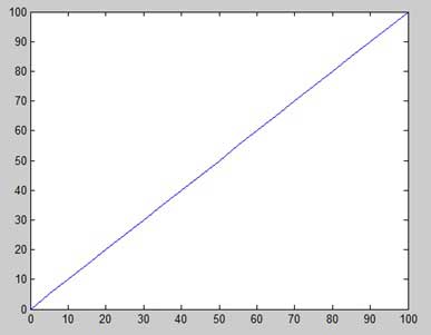
Following case would demonstrate the concept. Let u.s.a. plot the simple function y = ten for the range of values for x from 0 to 100, with an increase of 5.

Create a script file and type the following code −

x = [0:5:100]; y = x; plot(x, y)

When you lot run the file, MATLAB displays the following plot −

Plotting y = x

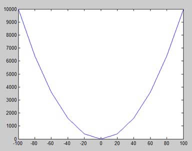
Let united states accept ane more than example to plot the office y = x². In this example, we will draw 2 graphs with the same function, but in second time, we will reduce the value of increase. Delight annotation that as we decrease the increment, the graph becomes smoother.

Create a script file and type the post-obit lawmaking −

ten = [1 2 3 4 5 6 7 8 9 x]; x = [-100:20:100]; y = x.^2; plot(x, y)

When you lot run the file, MATLAB displays the post-obit plot −

Plotting y = x^2

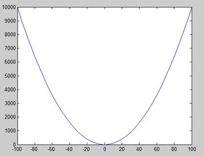
Change the lawmaking file a trivial, reduce the increase to five −

ten = [-100:5:100]; y = 10.^ii; plot(ten, y)

MATLAB draws a smoother graph −

Plotting y = x^2 with less increment

Calculation Championship, Labels, Filigree Lines and Scaling on the Graph

MATLAB allows you to add championship, labels along the x-axis and y-axis, grid lines and also to suit the axes to spruce up the graph.

The xlabel and ylabel commands generate labels along ten-axis and y-axis.
The championship command allows you lot to put a championship on the graph.
The filigree on command allows you to put the grid lines on the graph.
The axis equal control allows generating the plot with the same scale factors and the spaces on both axes.
The axis square command generates a square plot.

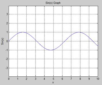
Instance

Create a script file and type the following code −

10 = [0:0.01:x]; y = sin(10); plot(x, y), xlabel('x'), ylabel('Sin(x)'), title('Sin(x) Graph'), grid on, axis equal

MATLAB generates the post-obit graph −

Sprucing up our graphs

Cartoon Multiple Functions on the Same Graph

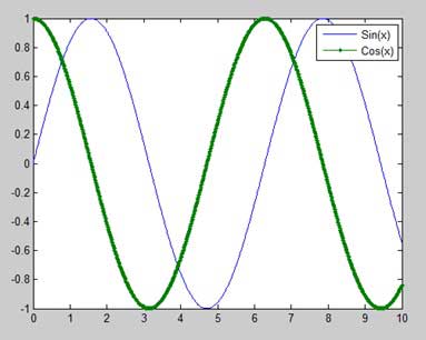
You can depict multiple graphs on the same plot. The following example demonstrates the concept −

Instance

Create a script file and type the post-obit code −

x = [0 : 0.01: 10]; y = sin(x); g = cos(10); plot(x, y, 10, chiliad, '.-'), legend('Sin(ten)', 'Cos(10)')

MATLAB generates the following graph −

Multiple Functions on the Same Graph

Setting Colors on Graph

MATLAB provides eight basic color options for cartoon graphs. The post-obit table shows the colors and their codes −

Code	Colour
w	White
k	Black
b	Blueish
r	Red
c	Cyan
g	Green
m	Magenta
y	Yellow

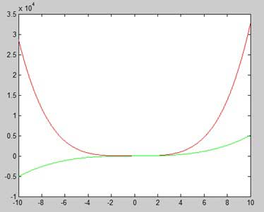
Example

Let us draw the graph of ii polynomials

f(x) = 3x⁴ + 2xⁱⁱⁱ+ 7x² + 2x + 9 and
yard(x) = 5x³ + 9x + ii

Create a script file and type the post-obit code −

x = [-10 : 0.01: 10]; y = 3*ten.^4 + two * ten.^3 + 7 * x.^two + ii * ten + 9; thousand = 5 * 10.^3 + ix * x + two; plot(ten, y, 'r', x, m, 'm')

When you lot run the file, MATLAB generates the following graph −

Colors on Graph

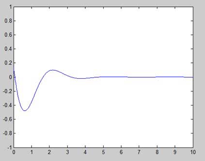
Setting Axis Scales

The centrality command allows you to set the axis scales. You can provide minimum and maximum values for 10 and y axes using the axis command in the following way −

centrality ( [xmin xmax ymin ymax] )

The following example shows this −

Example

Create a script file and blazon the following lawmaking −

10 = [0 : 0.01: 10]; y = exp(-x).* sin(2*x + 3); plot(x, y), centrality([0 10 -1 1])

When you lot run the file, MATLAB generates the following graph −

Setting Axis Scales

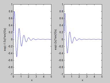
Generating Sub-Plots

When yous create an array of plots in the aforementioned figure, each of these plots is called a subplot. The subplot command is used for creating subplots.

Syntax for the command is −

subplot(m, n, p)

where, m and n are the number of rows and columns of the plot array and p specifies where to put a particular plot.

Each plot created with the subplot command can accept its own characteristics. Post-obit example demonstrates the concept −

Example

Let united states of america generate ii plots −

y = e^−1.5xsin(10x)

y = e^−2xsin(10x)

Create a script file and type the following code −

x = [0:0.01:five]; y = exp(-1.5*ten).*sin(10*ten); subplot(1,2,ane) plot(x,y), xlabel('x'),ylabel('exp(–1.5x)*sin(10x)'),axis([0 5 -1 1]) y = exp(-2*x).*sin(10*x); subplot(ane,2,2) plot(10,y),xlabel('10'),ylabel('exp(–2x)*sin(10x)'),centrality([0 5 -ane one])

When you run the file, MATLAB generates the following graph −

Generating Sub-Plots